Econ 265: Introduction to Econometrics
Lecture 2: Getting Started with R
Moshi Alam
Prerequisites
- R and RStudio is installed
- Update R packages regularly
- Required packages for today:
- Base R (primary focus)
Today’s Agenda
- Live coding
- Focus on typing commands yourself
- Avoid copy-paste to build muscle memory
Note
This is not a course in R!
RStudio Interface
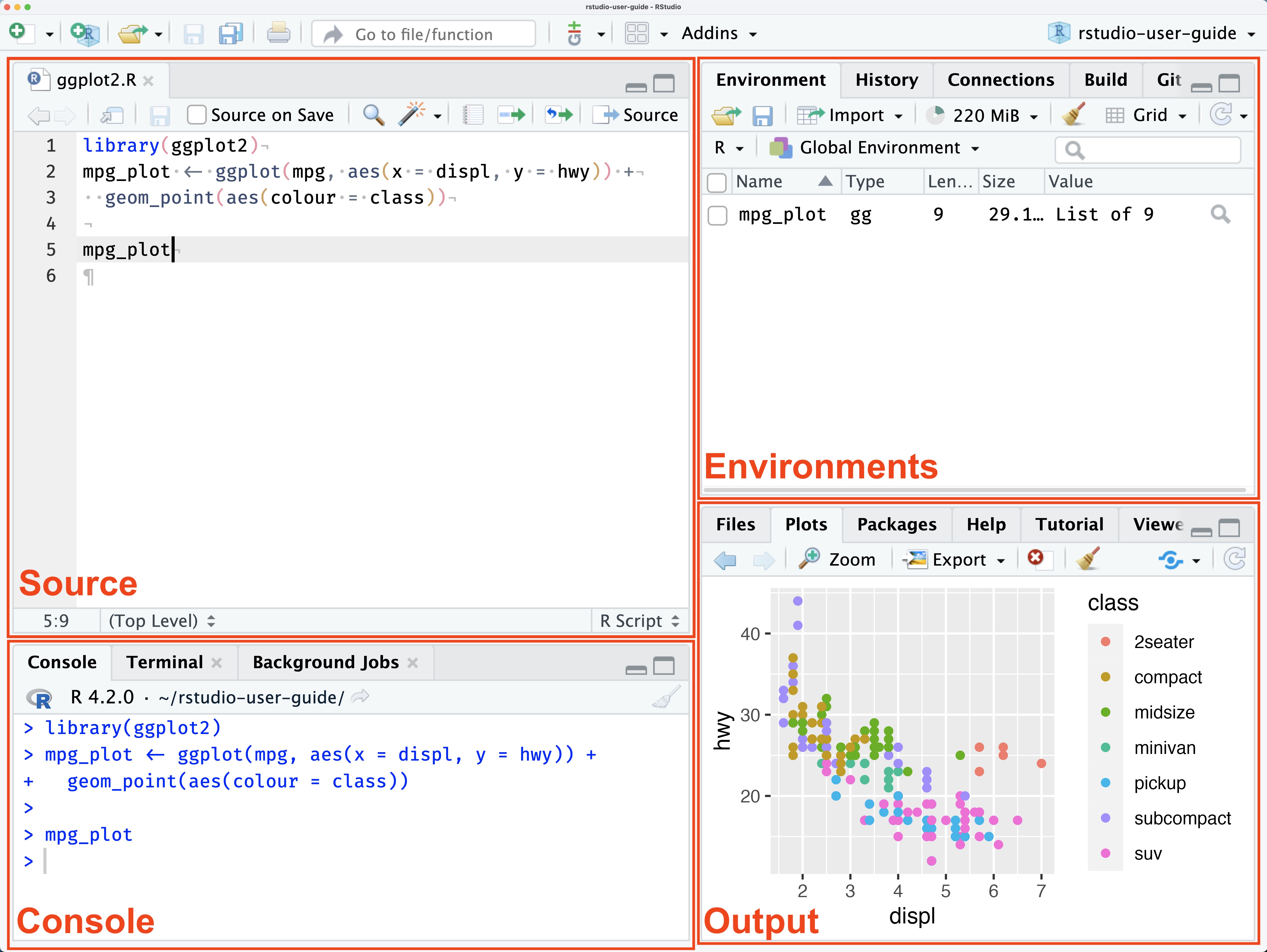
RStudio Interface
Basic Operations
Basic Arithmetic
Logic Operations
Logic: Important Details
Value Matching
Object-Oriented Programming
Everything is an Object
Common object types in R:
- Vectors
- Matrices
- Data frames
- Lists
- Functions
Objects Have Classes
Global Environment
Assignment
Assignment Operators
Using Arrow (<-):
Embodies the idea of assigned to
Assignment Choice
- Most R users prefer
<-for assignment =has specific role in function evaluation- Personal choice, but be consistent
=is quicker to type and familiar from other languages
Programming Basics
Variables and Assignment
Control Flow: if/else
Loops
Functions
Working with Variables
Creating Variables
Multiple Assignments
Data Types
Numeric Data
Text and Logical Data
Namespace Issues
Reserved Words
Namespace Conflicts
Two solutions:
- Use
package::function()
- Assign permanently
Indexing
Using Square Brackets
Using Dollar Sign
Cleaning Up
Removing Objects
Tip
Better to restart R session than use rm(list = ls())
Data Structures
Overview of Data Structures
R has several basic data structures:
| Dimension | Homogeneous | Heterogeneous |
|---|---|---|
| 1 | Vector | List |
| 2 | Matrix | Data Frame |
| 3+ | Array | nested Lists |
Vectors
Vectors are containers for objects of identical type:
Vector Operations
Vector Logic
Matrices
Two-dimensional arrays with same data type:
Matrix Operations
     [,1] [,2] [,3]
[1,]    2    6   10
[2,]    6   10   14
[3,] 10 14 18 [,1] [,2] [,3]
[1,] 1 8 21
[2,] 8 25 48
[3,] 21 48 81 [,1] [,2] [,3]
[1,] 66 78 90
[2,] 78 93 108
[3,] 90 108 126[1] 4[1] 1 4 7[1] 1 2 3Lists
Creating Lists
Lists can contain elements of different types:
List Operations
Packages
Installing Packages
Note
You only need to install a package once, but you need to load it each session
Help System
Getting Help
Data Frames
Introduction to Data Frames
Data frames are table-like structures:
Data Frame Operations
Subsetting Data Frames
Additional Resources
- R Documentation: r-project.org
- RStudio Cheatsheets: rstudio.com/resources/cheatsheets
- Advanced R by Hadley Wickham: adv-r.hadley.nz
- Stack Overflow R Tag: stackoverflow.com/questions/tagged/r
Practice on your own
- Create vectors using different methods (
c(),:,seq(),rep()) - Practice logical operations and understand operator precedence
- Create a list with different types of elements and practice indexing
- Load a package and resolve a namespace conflict
- Create and remove objects from your environment