library(wooldridge)
# gpa_model <- lm(colGPA ~ hsGPA, data = gpa1)
# summary(gpa_model)
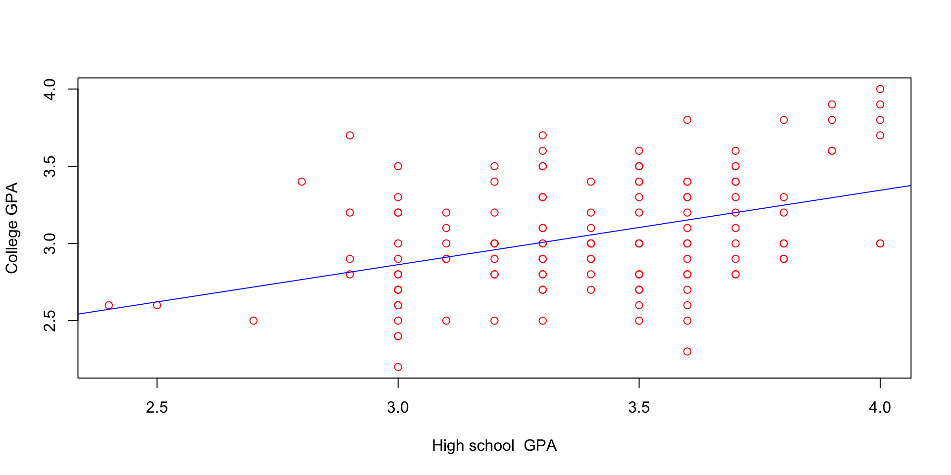
plot(gpa1$hsGPA, gpa1$colGPA,
xlab = "High school GPA",
ylab = "College GPA",
col = "red")
abline(lm(gpa1$colGPA ~ gpa1$hsGPA), col = "blue")
Topic 3: Simple Linear Regression
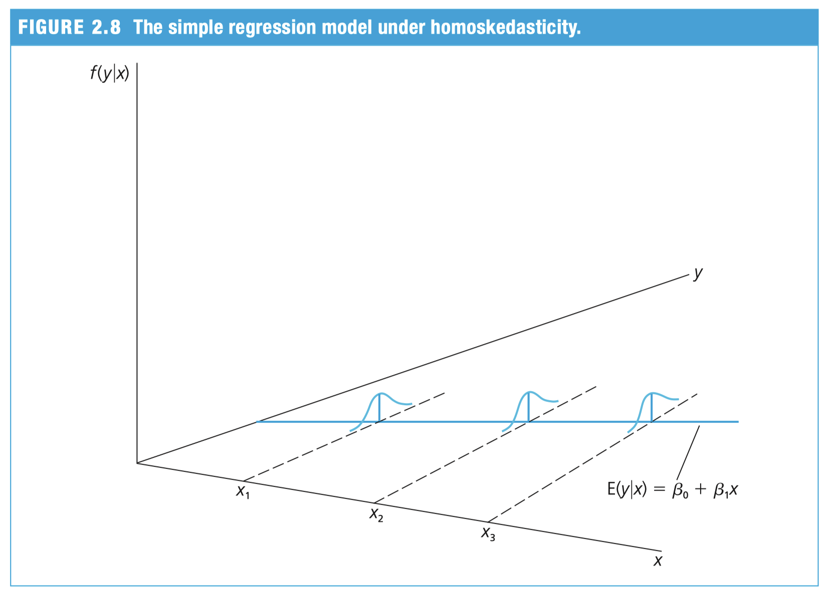
Zero conditional mean implies:
\(E(y_i|x_i) = \beta_0 + \beta_1x_i\)
Interpretation
gpa1 data
\(E(colGPA|hsGPA) = 1.5 + 0.5 \, hsGPA\)
For \(hsGPA = 3.6\):
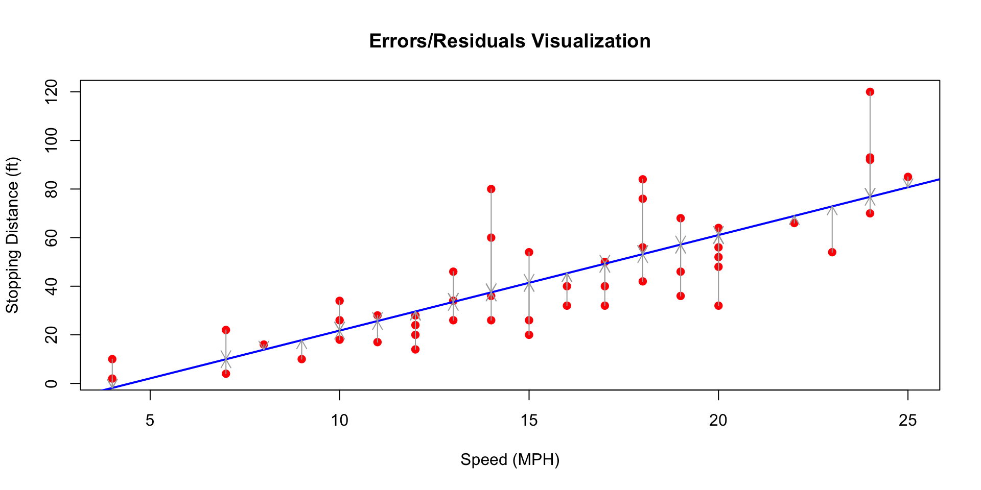
Systematic Part
Unsystematic Part
set.seed(123)
n <- 1e5
u1 <- rnorm(n, mean=0.0, sd=0.1)
x <- sin(seq(-5, 5, length.out=n))
u2 <- x + rnorm(n, mean=0, sd=0.1)
cat("Mean of u1:", mean(u1), "\n", "Mean of u2:", mean(u2), "\n")
Mean of u1: 9.767488e-05
Mean of u2: 0.0005215476 Try testing these out with this generated data:
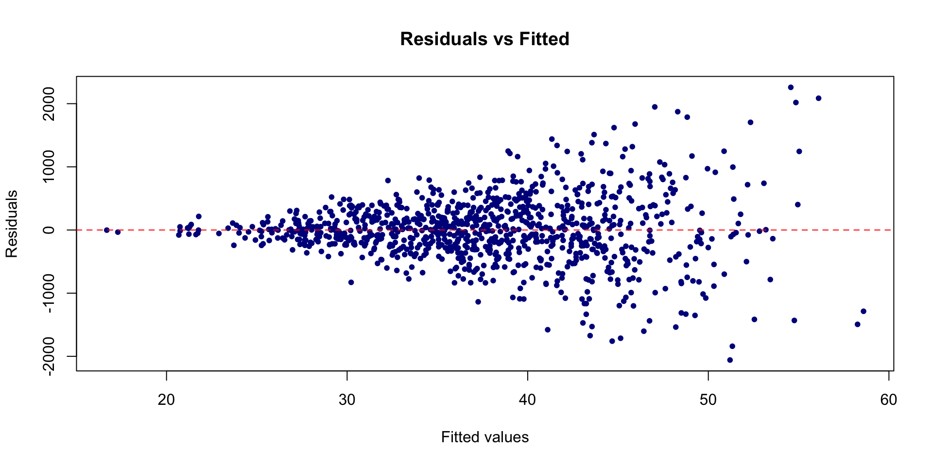
using Assumptions SLR. 4 and SLR. 5 we can derive the conditional variance of \(y\) :
\[ \begin{gathered} \mathrm{E}(y \mid x)=\beta_0+\beta_1 x \\ \operatorname{Var}(y \mid x)=\sigma^2 \end{gathered} \]
From here we can get \(Var(u \mid x)\)