You can explore the data in your own different ways.
Question 2
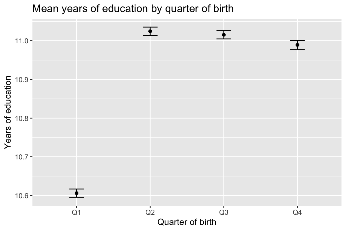
Shows evidence of a strong first stage
p1<-ggplot(dat, aes(qob, Educ))+stat_summary(fun =mean, geom ="point")+stat_summary(fun.data =mean_se, geom ="errorbar", width =0.2)+labs(title ="Mean years of education by quarter of birth", x ="Quarter of birth", y ="Years of education")print(p1)
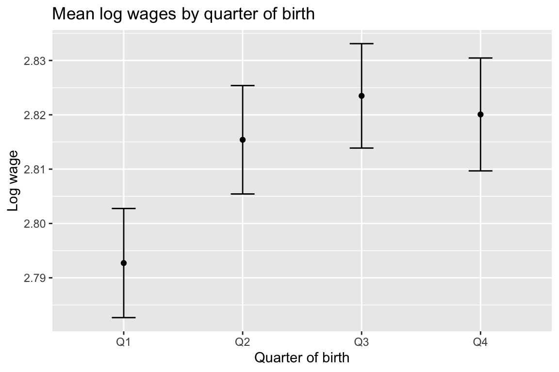
p2<-ggplot(dat, aes(qob, logwage))+stat_summary(fun =mean, geom ="point")+stat_summary(fun.data =mean_se, geom ="errorbar", width =0.2)+labs(title ="Mean log wages by quarter of birth", x ="Quarter of birth", y ="Log wage")print(p2)
Relevance: The first stage plot above shows that quarter of birth affects years of education. Specifically, being born in Q1 (Jan-Mar) leads to lower average years of education compared to other quarters. This is consistent with the idea that children born earlier in the year start school at a younger age and may drop out earlier, leading to fewer years of education on average.
Exogeneity: quarter of birth is potentially uncorrelated with unobservables that determine wages and are correlated with education There is no direct effect of quarter of birth on wages other than through education.
Question 4
first_stage<-lm(Educ~Z+age+factor(region), data =dat)summary(first_stage)
Call:
lm(formula = Educ ~ Z + age + factor(region), data = dat)

Residuals:
     Min       1Q   Median       3Q      Max
-1.33313 -0.24367 -0.00436  0.24341  1.27080

Coefficients:
                        Estimate Std. Error t value Pr(>|t|)
(Intercept)           11.9430837  0.0360378 331.404  < 2e-16 ***
Z                     -0.3991040  0.0116625 -34.221  < 2e-16 ***
age                   -0.0216297  0.0008488 -25.482  < 2e-16 ***
factor(region)Midwest -0.0709166  0.0152780  -4.642 3.54e-06 ***
factor(region)South   -0.1258614  0.0143128  -8.794  < 2e-16 ***
factor(region)West    -0.0338108  0.0163593  -2.067   0.0388 *
---
Signif. codes:  0 '***' 0.001 '**' 0.01 '*' 0.05 '.' 0.1 ' ' 1

Residual standard error: 0.3568 on 4994 degrees of freedom
Multiple R-squared:  0.2787,    Adjusted R-squared:  0.278
F-statistic: 385.9 on 5 and 4994 DF,  p-value: < 2.2e-16
Consistent with the plot, being born in Q1 reduces years of education by about 0.39 years on average, controlling for age and region fixed effects.
But we are not done, we have to test for weak IV, which we will do later.
Question 5
dat$Educ_hat<-fitted(first_stage)manual_second_stage<-lm(logwage~Educ_hat+age+region, data =dat)print(summary(manual_second_stage))
Call:
lm(formula = logwage ~ Educ_hat + age + region, data = dat)

Residuals:
    Min      1Q  Median      3Q     Max
-1.1855 -0.2423 -0.0007  0.2329  1.1525

Coefficients:
               Estimate Std. Error t value Pr(>|t|)
(Intercept)    1.742858   0.339489   5.134 2.95e-07 ***
Educ_hat       0.067000   0.028481   2.352 0.018691 *
age            0.010056   0.001036   9.707  < 2e-16 ***
regionMidwest -0.061907   0.015027  -4.120 3.86e-05 ***
regionSouth   -0.099866   0.014448  -6.912 5.38e-12 ***
regionWest    -0.054734   0.015970  -3.427 0.000614 ***
---
Signif. codes:  0 '***' 0.001 '**' 0.01 '*' 0.05 '.' 0.1 ' ' 1

Residual standard error: 0.3478 on 4994 degrees of freedom
Multiple R-squared:  0.03442,   Adjusted R-squared:  0.03345
F-statistic: 35.61 on 5 and 4994 DF,  p-value: < 2.2e-16
The average return to education is approximately 6.7% per additional year of education, controlling for age and region fixed effects when using quarter of birth as an instrument for education.
However, as discussed in class, the standard errors from this manual two-stage approach are not valid, since using the fitted values from the first stage does not account for the estimation error in the first stage.
We will address this using the ivreg function in the next question which will also allow us to formally test for weak IV.
Question 6
iv<-ivreg(logwage~Educ+age+region|Z+age+region, data =dat)summary(iv, diagnostics =TRUE)
Call:
ivreg(formula = logwage ~ Educ + age + region | Z + age + region,
    data = dat)

Residuals:
      Min        1Q    Median        3Q       Max
-1.134434 -0.230608 -0.003418  0.220237  1.111106

Coefficients:
                Estimate Std. Error t value Pr(>|t|)
(Intercept)    1.7428582  0.3230204   5.396 7.15e-08 ***
Educ           0.0669996  0.0270996   2.472 0.013456 *
age            0.0100564  0.0009858  10.201  < 2e-16 ***
regionMidwest -0.0619066  0.0142981  -4.330 1.52e-05 ***
regionSouth   -0.0998656  0.0137475  -7.264 4.33e-13 ***
regionWest    -0.0547343  0.0151953  -3.602 0.000319 ***

Diagnostic tests:
                  df1  df2 statistic p-value
Weak instruments    1 4994    1171.1  <2e-16 ***
Wu-Hausman          1 4993     850.2  <2e-16 ***
Sargan              0   NA        NA      NA
---
Signif. codes:  0 '***' 0.001 '**' 0.01 '*' 0.05 '.' 0.1 ' ' 1

Residual standard error: 0.3309 on 4994 degrees of freedom
Multiple R-Squared: 0.1258, Adjusted R-squared: 0.125
Wald test: 39.33 on 5 and 4994 DF,  p-value: < 2.2e-16
The corresponding F-stat is more than a thousand, so we can reject the null of weak instrument.
The IV estimate of the return to education is approximately 6.7% per additional year of education, controlling for age and region fixed effects, but now with correct standard errors.
Question 7
This is an estimate of the local average treatment effect (LATE) for compliers affected by the instrument i.e., those whose education decisions are influenced by their quarter of birth.
This is because only for those individuals whose education is affected by the instrument (compliers), the instrument uses the exogenous variation to identify the causal effect of education on wages.